Voronoi diagram and Dealunay triangulation construction of Big Spatial Data using SpatialHadoop

Voronoi Diagram and Delaunay Triangulation

A very popular computational geometry problem is the Voronoi Diagram (VD), and its dual Delaunay Triangulation (DT). In both cases, the input is a set of points (sites). In VD, the output is a tessellation of the space into convex polygons, as one per input site, such that each polygon covers all locations that are closest to the corresponding site than any other site. In DT, the output is a triangulation, where each triangle connects three sites, such that the circumcirlce of each triangle does not contain any other sites. These two constructs are dual in a sense that each edge in the DT connects two sites that share a common edge in VD.

Computation Overhead

These two problems, DT and VD, are known to be computationally intensive. There are several O(n log n) algorithms for both but they are mainly single-machine main-memory algorithms and cannot scale to the current sizes of Big Spatial Data. For example, earth surface modeling is usually done via Delaunay triangulation of elevation data. With the increasing resolution of data collected through LiDAR, we might need to construct a Delaunay triangulation for a few trillions of points which cannot be loaded into one machine.

SpatialHadoop and CG_Hadoop

SpatialHadoop provides a computational geometry library, named CG_Hadoop, which includes MapReduce algorithms for both VD and DT. These algorithms can scale to trillions of points by distributing the computation over a Hadoop cluster with up-to thousands of machines. SpatialHadoop is able to construct a DT of 2.7 billion points extracted from OpenStreetMap in less than an hour using only 20 machines.

Single-machine Divide and Conquer (D&C) Algorithm

SpatialHadoop MapReduce algorithm is based on the  main-memory divide and conquer algorithm. This traditional algorithm, originally proposed by Guibas and Stolfi, divides the input sites into two subsets using a straight line, usually a vertical line, computes the DT recursively for each subset, and then merges the two partial DTs. This algorithm requires all data to fit in the main memory which cannot be done with big spatial datasets.

CG_Hadoop MapReduce Algorithm

A straight forward implementation of the D&C algorithm in MapReduce wouldn't work because of the overhead of the merge step. The final merge step has to be done on a single machine and it would require loading the whole final DT in its main memory, which takes us back to the limitation of the single-machine algorithm. Alternatively, CG_Hadoop proposes a novel approach which employs the following two techniques:

1. Instead of partitioning the space into two, CG_Hadoop partitions the space using one of the SpatialHadoop partitioning methods, e.g., Grid or R-tree, so that it achieves a higher level of parallelism by assigning each partition to one of the machines.
2. CG_Hadoop early detects VD portions that are final, i.e., will never be affected or used by subsequent merge process. In other words, CG_Hadoop detects the Voronoi regions, or Delaunay triangles, that might be affected by the merge step, and only sends these portions to the merge step.

These two techniques allow the construction process of both VD and DT to be much more scalable as each machine computes a partial VD one partition at a time. Then, each machine early detects parts of the partial VD that will not be affected by the subsequent merge steps, and early writes them to the output. Furthermore, the merge step becomes much faster and scalable as it deals with only a few non-final parts of the VD rather than all of it.

The figure below illustrates the main idea of the pruning technique. The input points are partitioned using a uniform grid into four partitions. The VD of each partition is computed on a separate machine in the map function. Each machine detects final Voronoi regions, marked in green, and writes them to the final output. Only non-final regions, marked in red, are sent to the next merge step.

Local VD step. Each mapper computes a partial VD for one partition and writes final Voronoi Regions (green) to the output. Non-final regions (red) are sent to the next step for merging

How to Use it

The above algorithm ships with the recent version of SpatialHadoop available on github. First, you need to spatially partition the input set of points using the 'index' command. For example

shadoop index input.points shape:point input.grid sindex:grid

Then, you will call the DT operation as follows:

shadoop dt input.grid output.dt shape:point

It launches a single MapReduce job that generates the DT of the input set of points.

More Details

The VD algorithm runs in four steps, namely, partitioning, local VD, vertical merge, and horizontal merge.

1. Partitioning

The partitioning step uses any space partitioning technique supported by SpatialHadoop, such as a uniform grid index.

2. Local VD

In the local VD step, each partition is assigned to one machine which computes the VD for all points in that partition. We use the traditional Guibas and Stolfi D&C algorithm as the size of each partition is small enough to fit in the main memory. We can also use a more advanced algorithm, such as Dwyer's algorithm. We leave this as an exercise for interested readers. Upon the computation of the local VD, each machine detects final Voronoi regions, removes them from the VD, and writes them to the final output. To detect final regions, we use a very simple, yet efficient, rule that is derived from the VD definition. Simply, a Voronoi region is final if it is not possible to have any other point closer to its generator site. The following figure shows two examples of final and non-final regions.

A final Voronoi region. The nearest possible site outside the partition is still farther away than the generator site of that region

A non-final Voronoi region. There could be a site (S2) in another partition that is closer to some (shaded) areas in that Voronoi region.

To find all non-final regions quickly, without exhaustively applying this rule to all regions, we run a breadth-first search (BFS) from the outer regions which expands only to non-final regions. The trick is that all non-final regions form a contiguous region towards the exterior of the VD. In this way, a VD of 1.4 million regions can be pruned by applying the rule to only 7K regions.

3. Vertical Merge

In this step, partial VDs which are on the same column of the partition grid are merged together into vertical strips. This step can be done in parallel as each machine is assigned all partial VDs in one vertical strip. Notice that each machine receives only non-final regions from the assigned VDs are processed by that machine which reduces the memory and computation overhead. After merging them, the pruning rule is applied again to further remove final regions that will not be processed later, as shown in the figure below.

The vertical merge step. Each vertical strip is processed by a reducer which merges all partial VDs in that strip. Final regions in the strip (blue) are directly written to the output while non-final regions (red) are sent to the next step for the final merge step.

4. Horizontal Merge

In this final step, all partial VDs computed for vertical strips are sent to one machine which merges them to compute the final answer. Again, only non-final regions are processed at this step which makes it possible to run on a single machine. As shown in the figure below, all resulting regions are written to disk as there is no further merge steps.

The final horizontal merge step. All resulting Voronoi regions are written to the final output as there are no further merge step.

The Voronoi regions written by the three steps comprise the final VD, as shown in the figure below.

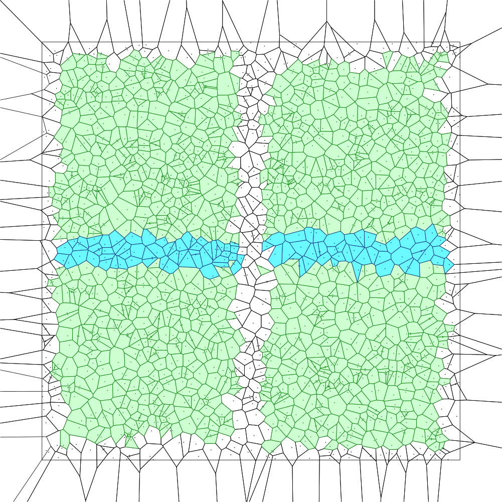The final results. Green, blue and black regions are the ones written by the local VD, vertical merge, and horizontal merge steps, respectively.

Performance Evaluation

We run the above algorithm on Amazon EC2 using a real dataset extracted from OpenStreetMap. We compare to the standard D&C algorithm running on a machine with 1TB of memory. We have access to such a powerful machine through Minnesota Supercomputing Institute (MSI). CG_Hadoop is 30 times faster than a single machine with 1 billion points. Furthermore, the single machine fails to process the 2.7 billion dataset while CG_Hadoop finishes the computation in around 40 minutes.

Acknowledgement

The work in Voronoi diagrams was done with Nadezda Weber while she was studying in University of Minnesota. She is currently a graduate student in Oxford University.
The experiments were run on an Amazon EC2 cluster and were supported by AWS in Education Grant award.

External Links

• SpatialHadoop: A MapReduce Framework for Spatial Data
• Voronoi Diagram/Delaunay Triangulation Applet